From Circles to Waveforms
A simple, visual introduction to sine, square, triangle, sawtooth, pulse and noise synthesis. Periodic waveforms are built from rotating sine waves added together; noise introduces random / stochastic values.
The equations are included for reference. We do not need to understand the notation to understand the synthesis principle.
1. Start with a clock: the sine wave
Imagine a point moving around a circle at a constant speed. One complete trip around the circle is one complete cycle.
The idea
If we trace only the point's vertical position while the point travels around the circle, the trace becomes a sine wave.
A = amplitude • f = frequency • t = time • φ = phase • 2π = one complete rotation
2. Add sine waves together
A more complex periodic waveform can be built by adding sine waves with different frequencies, amplitudes and phases.
The large Greek letter Σ (sigma) simply means: repeat this rule and add the results together.
In digital audio we only include harmonics that fit below the Nyquist frequency. At a 48 kHz sample rate, Nyquist is 24 kHz.
3. The six basic waveform recipes
one frequency
odd harmonics
1/n amplitude
odd harmonics
1/n² amplitude
all harmonics
1/n amplitude
all possible harmonics
set by pulse width
random values
spectral shaping
4. Square wave
Use the fundamental, then the odd harmonics: 1st, 3rd, 5th, 7th… Their amplitudes fall as 1, 1/3, 1/5, 1/7…
With only a few harmonics the shape is rounded. Add more and the flat tops and steep edges become clearer. A mathematically perfect vertical edge would require infinitely many harmonics, which a real digital system cannot contain.
In practical digital oscillator design we therefore do not normally create an infinitely sharp mathematical discontinuity and simply hope for the best. Band-limited techniques such as wavetables, BLEP and PolyBLEP can be used to retain the character of a square wave while controlling harmonics that would otherwise exceed Nyquist and alias.
5. Triangle wave
Again use odd harmonics, but the upper harmonics get quiet much faster: 1, 1/9, 1/25, 1/49… Alternate their sign and the summed result becomes a triangle.
This rapid high-frequency fall-off is why a triangle sounds softer than a square.
6. Sawtooth wave
A saw uses all integer harmonics: 1st, 2nd, 3rd, 4th, 5th… Their amplitudes fall approximately as 1/n.
An upward and downward saw are polarity opposites: multiply the waveform by −1 to flip it.
7. Pulse wave
A pulse wave spends one part of each cycle high and the remainder low. Its duty cycle (or pulse width) determines the harmonic balance.
D is the duty cycle, from 0 to 1. This compact rule tells us how much of each harmonic is needed.
8. Noise
Noise is different from the repeating waveforms above. Instead of tracing a repeating cycle, we generate a new value at each sample.
For white noise, each sample is independent of the previous one. The result is a random-looking waveform whose ideal power spectral density is flat: equal power per Hz of bandwidth.
Time domain
Simplified spectrum
| Noise | Spectral idea | Simple description |
|---|---|---|
| White | Flat power per Hz | Equal power in equal-width frequency bands. |
| Pink | ~ −3 dB/octave | Equal power per octave; often sounds more balanced to us. |
| Brown / red | ~ −6 dB/octave | More strongly weighted toward low frequencies. |
The spectrum display is deliberately simplified to show the expected overall slope rather than a detailed FFT of one short random sequence.
9. One idea, six synthesis ideas
| Waveform | Harmonics | Amplitude rule | Main idea |
|---|---|---|---|
| Sine | Fundamental only | One amplitude | One rotating point |
| Square | Odd only | 1/n | Add odd sine waves |
| Triangle | Odd only | 1/n², alternating sign | Upper harmonics fade faster |
| Sawtooth | All harmonics | 1/n | Every integer harmonic contributes |
| Pulse | Depends on width | sin(πnD)/n | Pulse width controls the spectrum |
| Noise | Broadband / stochastic | Random values + spectral shaping | No repeating cycle is required |
Periodic waveforms can be described as sine-wave components. Each component has a frequency, amplitude and phase. Fourier synthesis adds those components together; Fourier analysis works in the opposite direction and tells us which components are present. Noise adds a second basic synthesis idea: generate stochastic values, then shape their spectrum if required.
Digital audio version
Choose a fundamental frequency → generate the required harmonics → set each harmonic's amplitude and phase → stop before Nyquist → sum the components → scale the final waveform to the desired amplitude.
We have constructed these waveforms by adding sine-wave harmonics because Fourier synthesis makes their internal frequency structure easy to see and understand. A practical digital synthesiser does not necessarily generate them this way. Calculating many separate sinusoidal components for every sample can be computationally inefficient. Digital oscillators may instead use techniques such as lookup tables, band-limited wavetables, BLEP or PolyBLEP, depending on the oscillator design. The waveform can still be described by the same Fourier components even though those components were not individually generated and summed.
10. Analogue generation — a different route
We have constructed these waveforms by adding sine-wave harmonics because Fourier synthesis makes their internal frequency structure easy to see and understand. However, a practical digital synthesiser does not necessarily generate them this way.
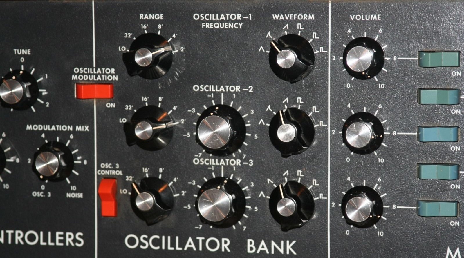
In analogue electronics, producing ramps, pulses and square-like waveforms can be relatively simple. Producing a very pure sine wave may require additional shaping.
In digital synthesis, generating a sine wave is straightforward, while producing a sharp square or sawtooth without aliasing requires more care.
The charging capacitor
One common analogue oscillator design uses a capacitor. A capacitor can be thought of as a small electrical bucket. If it is charged at a controlled rate, its voltage changes progressively through time.
That changing voltage can itself become the basis of an oscillator.
Sawtooth — charge and reset
To generate a sawtooth-like waveform, the capacitor is allowed to charge until its voltage reaches a threshold. A circuit then rapidly resets the capacitor and the process begins again.
Plot the capacitor voltage against time and we obtain the characteristic rising ramp followed by a rapid drop.
Square and pulse — compare against a threshold
Once we have a changing voltage such as a ramp, a comparator provides a very simple way of generating a two-state waveform.
The comparator therefore switches rapidly between two voltage states, producing a square or pulse waveform.
With a centred threshold we can obtain approximately 50% duty cycle. Move the threshold and the proportion of HIGH and LOW changes, producing different pulse widths. Later, if we continuously move that threshold with another control signal, we obtain pulse-width modulation (PWM).
Why does analogue not have the same Nyquist problem?
A purely analogue oscillator is continuous in time. At this stage there is no digital sample rate and therefore no digital Nyquist frequency for the oscillator to exceed.
This does not mean analogue electronics have infinite bandwidth or perfectly instantaneous edges. Real components have finite bandwidth and non-zero transition times, which naturally limit their highest-frequency behaviour.
Once that analogue waveform is sampled by a digital system, however, Nyquist becomes important again and frequencies above the permitted range must be appropriately controlled.
The digital square-wave problem
In code, creating a mathematically abrupt square wave is extremely easy:
The problem is that an instantaneous discontinuity implies harmonics extending indefinitely. In a sampled system, harmonics above Nyquist can fold back into the audible range as aliasing.
As such, digital oscillators commonly use band-limited techniques such as precomputed band-limited wavetables, BLIT, BLEP or PolyBLEP. These methods preserve the useful character of a square or sawtooth while reducing the unwanted above-Nyquist components.
Fourier tells us what the waveform contains.
Analogue circuitry and digital algorithms may generate that waveform in very different ways.
| Relatively straightforward | Requires more care | |
|---|---|---|
| Analogue | Ramp / square / pulse | Very pure sine |
| Digital | Pure sine | Sharp alias-free ramp / square / pulse |